IAS Demo

This is a demo for testing the Iterative Alternating Sequential (IAS) algorithm.

The real data set used for this demo is the MEG sample data acquired with the Neuromag Vectorview system at MGH/HMS/MIT Athinoula A. Martinos Center Biomedical Imaging and made available, together with the MRI reconstructions created with FreeSurfer, in the MNE python software package.

As part of the protocol for the data collection, checkerboard patterns were presented into the left and right visual field, interspersed by tones to the left or right ear. The interval between the stimuli was 750 ms. Occasionally a smiley face was presented at the center of the visual field. The subject was asked to press a key with the right index finger as soon as possible after the appearance of the fac.e [Ref] Here we only consider the trials corresponding to the left visual stimulus and perform the averaging on these trials. The source space containing both cortical regions and subcortical structures after discretization comprises 19054 vertices.

Note

Click here to download the data for IAS demo.

Ref

1. Gramfort et al, MNE software for processing MEG and EEG data, Neuroimage 86 (2014) 446-460

%% Reset all
clear; clc;
close all

%% Input
%     SNR: estimated signal-to-noise ratio
SNR = 9;
%     eta: scalar, parameter for selecting the focality of the reconstructed activity
eta = 0.01;
cut_off = 0.9;

%% Loading the source space
%     coord, normals: (3,N) array, coordinates and normal vectors of the dipoles in the grid
disp('Loading source space')
load('SourceSpace_DBA')

%% Loading the leadfield matrix
%     LF: (M,3*N) array, the lead field matrix (M is the number of channels; N is the number of dipoles)
disp('Loading leadfield matrix')
load('LeadfieldMatrix_DBA')

%% Loading the magnetic data
%     data: (M,T) array, a set of data of length T
%     time: T-vector, times
disp('Loading data')
load('visualMEGData')

%% Building anatomical prior
:func:`IAS.BuildAnatomicalPrior`
disp('Building anatomical prior')
APChol = BuildAnatomicalPrior(coord,normals);

%% Setting theta_star and scaling
disp('Setting parameters')
t_peak = 86;
t_min = 1;
t_max = 211;
B = data(:,t_min:t_max);
[theta_star,theta_cut_off,sigma,LF_scaling,B_scaling] = SetParameters(LF,APChol,B,SNR,cut_off);

%% Solving the inverse problem using IAS algorithm
disp(['Running IAS algorithm from time ',num2str(time(t_min)),' ms to time ',num2str(time(t_max)),' ms'])
Q = IAS_algorithm(LF, LF_scaling, APChol, B, B_scaling, sigma, theta_star, eta);

%% Visualizing the activity map
disp(['Visualizing activity map at time ',num2str(time(t_peak)),' ms'])
N = size(LF,2)/3;  % number of dipoles in the source space
t_vis = t_peak - t_min + 1;
q = Q(:, t_vis);
dip_norm2 = sum(reshape(q,3,N).^2,1);
Q_est = sqrt(dip_norm2);
SlicedVisualization_ActivityMap(coord,Q_est);

%% Visualazing the activity map and its maximum
[Q_max,i_max] = max(Q_est);
r0 = coord(:,i_max);
SingleSliceVisualization_ActivityMap(coord,Q_est,r0,'CoordSystem','Brainstorm','ColorScale','double','Locator','pinhead');

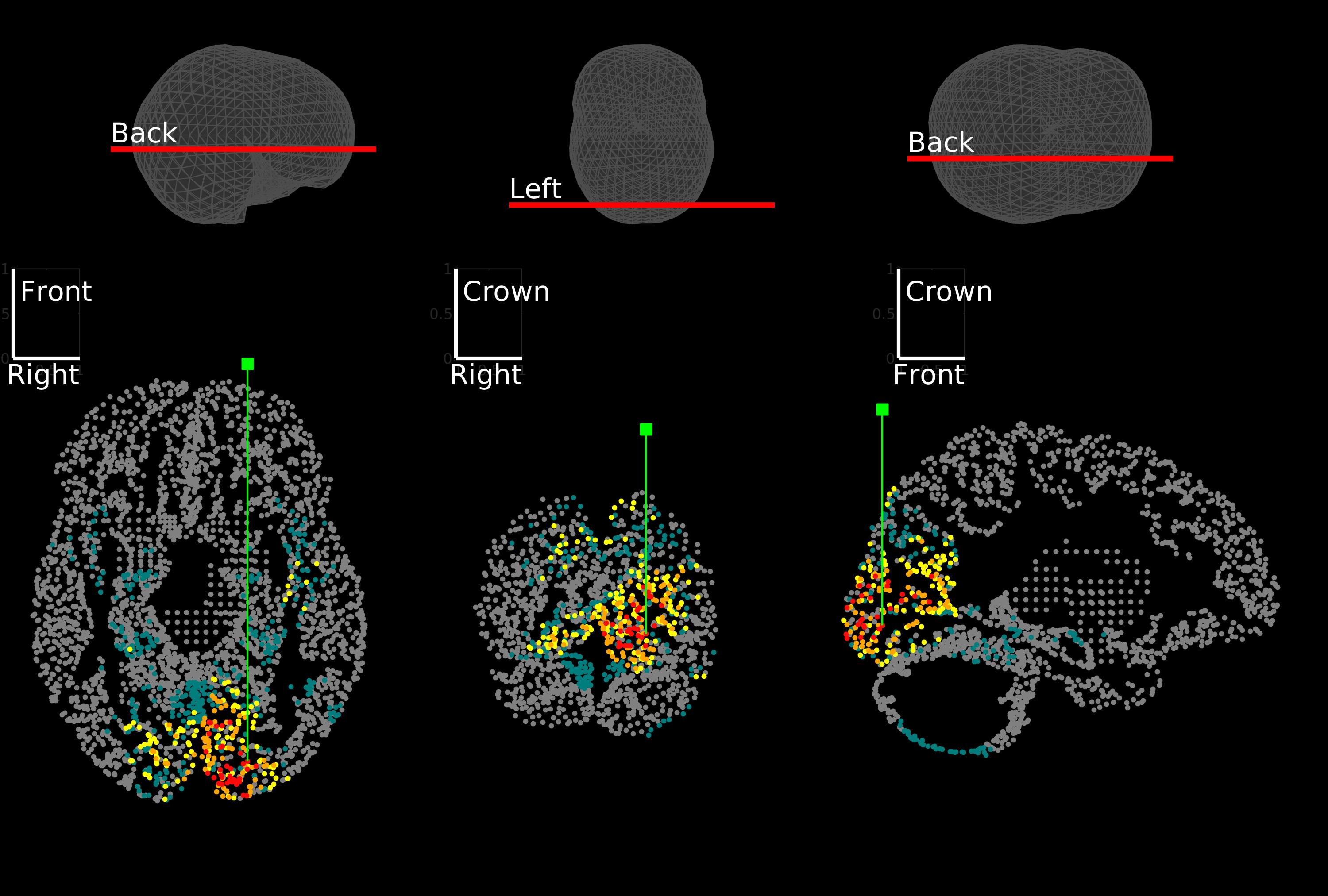
Reconstructed activity map from real data at 92 ms

Download IAS Demo script: IAS_Demo.m